What is Julia? A fresh approach to numerical computing
Julia is a free open source, high-level, high-performance, dynamic programming language for numerical computing. It has the development convenience of a dynamic language with the performance of a compiled statically typed language, thanks in part to a JIT-compiler based on LLVM that generates native machine code, and in part to a design that implements type stability through specialization via multiple dispatch, which makes it easy to compile to efficient code.
In the blog post announcing the initial release of Julia in 2012, the authors of the language—Jeff Bezanson, Stefan Karpinski, Viral Shah, and Alan Edelman—stated that they spent three years creating Julia because they were greedy. They were tired of the trade-offs among Matlab, Lisp, Python, Ruby, Perl, Mathematica, R, and C, and wanted a single language that would be good for scientific computing, machine learning, data mining, large-scale linear algebra, parallel computing, and distributed computing.
Who is Julia for? In addition to being attractive to research scientists and engineers, Julia is also attractive to data scientists and to financial analysts and quants.
The designers of the language and two others founded Julia Computing in July 2015 to “develop products that make Julia easy to use, easy to deploy, and easy to scale.” As of this writing, the company has a staff of 28 and customers ranging from national labs to banks to economists to autonomous vehicle researchers. In addition to maintaining the Julia open source repositories on GitHub, Julia Computing offers commercial products, including JuliaPro, which comes in both free and paid versions.
Why Julia?
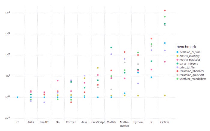
Julia “aims to create an unprecedented combination of ease-of-use, power, and efficiency in a single language.” To the issue of efficiency, consider the graph below:
 Julia Computing
The figure above shows performance relative to C for Julia and 10 other languages. Lower is better. The benchmarks shown are very low-level tasks. The graph was created using the Gadfly plotting and data visualization system in a Jupyter notebook. The languages to the right of Julia are ordered by the geometric mean of the benchmark results, with LuaJIT the fastest and GNU Octave the slowest.
Julia benchmarks
What we’re seeing here is that Julia code can be faster than C for a few kinds of operations, and no more than a few times slower than C for others. Compare that to, say, R, which can be almost 1,000 times slower than C for some operations.
Note that one of the slowest tests for Julia is Fibonacci recursion; that is because Julia currently lacks tail recursion optimization. Recursion is inherently slower than looping. For real Julia programs that you want to run in production, you’ll want to implement the loop (iteration) form of such algorithms.
Julia JIT compilation
There is a cost to the JIT (just-in-time) compiler approach as opposed to a pure interpreter: The compiler has to parse the source code and generate machine code before your code can run. That can mean a noticeable start-up time for Julia programs the first time each function and macro runs in a session. So, in the screenshot below, we see that the second time we generate a million random floating point numbers, the time taken is an order of magnitude less than on the first execution. Both the @time macro and the rand() function needed to be compiled the first time through the code, because the Julia libraries are written in Julia.
julia> @time rand(10^6);
0.62081 seconds (14.44 k allocations: 8.415 MiB)julia> @time rand(10^6);
0.004881 seconds (7 allocations: 7.630 MiB)
Julia fans claim, variously, that it has the ease of use of Python, R, or even Matlab. These comparisons do bear scrutiny, as the Julia language is elegant, powerful, and oriented towards scientific computing, and the libraries supply a broad range of advanced programming functionality.
Julia example
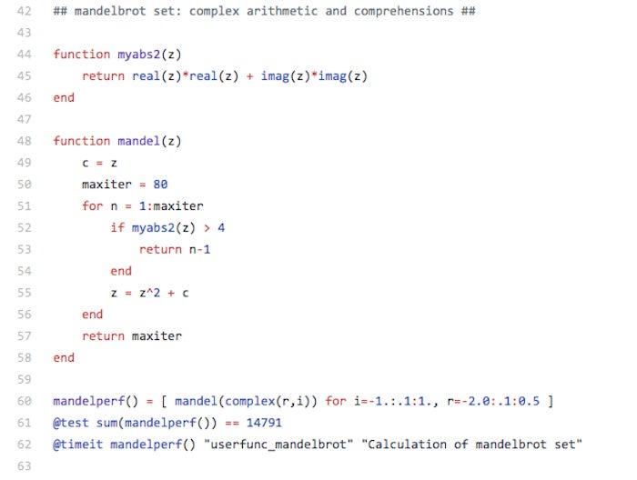
As a quick Julia language example, consider the following Mandelbrot set benchmark code:
 IDG
IDG
Mandelbrot set benchmark in Julia.
As you can see, complex number arithmetic is built into the language, as are macros for tests and timing. As you can also see, the trailing semicolons that plague C-like languages, and the nested parentheses that plague Lisp-like languages, are absent from Julia. Note that mandelperf() is called twice, in lines 61 and 62. The first call tests the result for correctness and does the JIT-compilation; the second call gets the timing.
Julia programming
Julia has many other features worth mentioning. For one, user-defined types are as fast and compact as built-ins. In fact, you can declare abstract types that behave like generic types, except that they are compiled for the argument types that they are passed.
For another, Julia’s built-in code vectorization means that there is no need for a programmer to vectorize code for performance; ordinary devectorized code is fast. The compiler can take advantage of SIMD instructions and registers if present on the underlying CPU, and unroll the loops in a sequential process to vectorize them as much as the hardware allows. You can mark loops as vectorizable with the @simd annotation.
Julia parallelism
Julia was also designed for parallelism and distributed computation, using two primitives: remote references and remote calls. Remote references come in two flavors: Future and RemoteChannel. A Future is the equivalent of a JavaScript promise; a RemoteChannel is rewritable and can be used for inter-process communication, like a Unix pipe or a Go channel. Assuming that you have started Julia with multiple processes (e.g. julia -p 8 for an eight-core CPU such as an Intel Core i7), you can @spawn or remotecall() function calls to execute on another Julia process asynchronously, and later fetch() the Future returned when you want to synchronize and use the result.
If you don’t need to run on multiple cores, you can utilize lightweight “green” threading, called a Task() in Julia and a coroutine in some other languages. A Task() or @task works in conjunction with a Channel, which is the single-process version of RemoteChannel.
Julia type system
Julia has an unobtrusive yet powerful type system that is dynamic with run-time type inference by default, but allows for optional type annotations. This is similar to TypeScript. For example:
julia> (1+2)::AbstractFloat
ERROR: TypeError: typeassert: expected AbstractFloat, got Int64
julia> (1+2)::Int
3
Here we are asserting an incompatible type the first time, causing an error, and a compatible type the second time.
Julia strings
Julia has efficient support for Unicode strings and characters, stored in UTF-8 format, as well as efficient support for ASCII characters, since in UTF-8 the code points less than 0x80 (128) are encoded in a single character. Otherwise, UTF-8 is a variable-length encoding, so you can’t assume that the length of a Julia string is equal to the last character index.
Full support for UTF-8 means, among other things, that you can easily define variables using Greek letters, which can make scientific Julia code look very much like the textbook explanations of the formulas, e.g. sin(2π). A transcode() function is provided to convert UTF-8 to and from other Unicode encodings.
C and Fortran functions
Julia can call C and Fortran functions directly, with no wrappers or special APIs needed, although you do need to know the “decorated” function name emitted by the Fortran compiler. The external C or Fortran function must be in a shared library; you use the Julia ccall() function for the actual call out. For example, on a Unix-like system you can use this Julia code to get an environment variable’s value using the getenv function in libc:
function getenv(var::AbstractString)
val = ccall((:getenv, "libc"),
Cstring, (Cstring,), var)
if val == C_NULL
error("getenv: undefined variable: ", var)
end
unsafe_string(val)
endjulia> getenv("SHELL")
"/bin/bash"
Julia macros
Julia has Lisp-like macros, as distinguished from the macro preprocessors used by C and C++. Julia also has other meta-programming facilities, such as reflection, code generation, symbol (e.g. :foo) and expression (e.g. :(a+b*c+1) ) objects, eval(), and generated functions. Julia macros are evaluated at parsing time.
Generated functions, on the other hand, are expanded when the types of their parameters are known, prior to function compilation. Generated functions have the flexibility of generic functions (as implemented in C++ and Java) and the efficiency of strongly typed functions, by eliminating the need for run-time dispatch to support parametric polymorphism.
GPU support
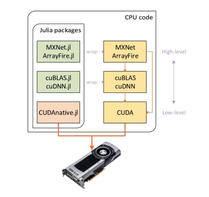
Julia has GPU support using, among others, the MXNet deep learning package, the ArrayFire GPU array library, the cuBLAS and cuDNN linear algebra and deep neural network libraries, and the CUDA framework for general purpose GPU computing. The Julia wrappers and their respective libraries are shown in the diagram below.
 Julia Computing
You can draw on a number of Julia packages to program GPUs at different abstraction levels.
JuliaPro and Juno IDE
You can download the free open source Julia command line for Windows, MacOS, generic Linux, or generic FreeBSD from the Julia language site. You can clone the Julia source code repository from GitHub.
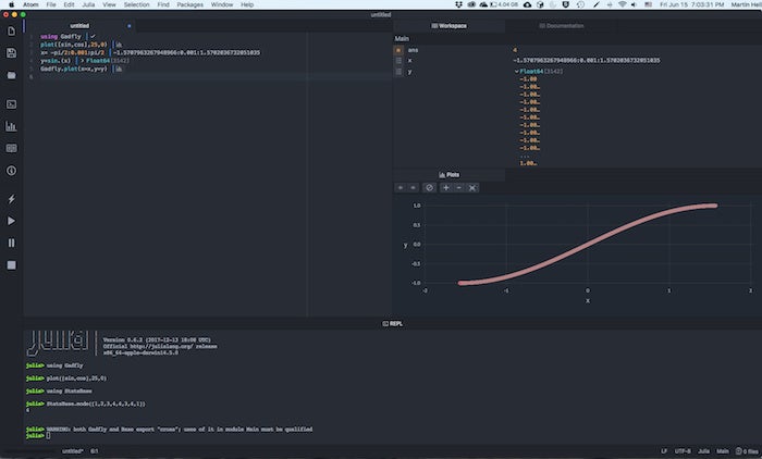
Alternatively you can download JuliaPro from Julia Computing. In addition to the compiler, JuliaPro gives you the Atom-based Juno IDE (shown below) and more than 160 curated packages, including visualization and plotting.
Beyond what’s in the free JuliaPro, you can add subscriptions for enterprise support, quantitative finance functionality, database support, and time series analysis. JuliaRun is a scalable server for a cluster or cloud.
 IDG
IDG
Juno is a free Julia IDE based on the Atom text editor.
Jupyter notebooks and IJulia
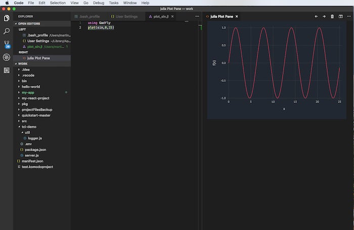
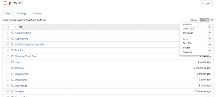
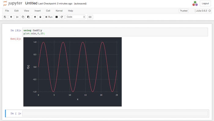
In addition to using Juno as your Julia IDE, you can use Visual Studio Code with the Julia extension (shown directly below), and Jupyter notebooks with the IJulia kernel (shown in the second and third screenshots below). You may need to install Jupyter notebooks for Python 2 or (preferably) Python 3 with Anaconda or pip.
 IDG
IDG
Visual Studio Code with the Julia extension.
 IDG
IDG
Launching a Julia kernel from Jupyter notebook.
 IDG
IDG
Plotting a sine wave using Julia in a Jupyter notebook.
JuliaBox
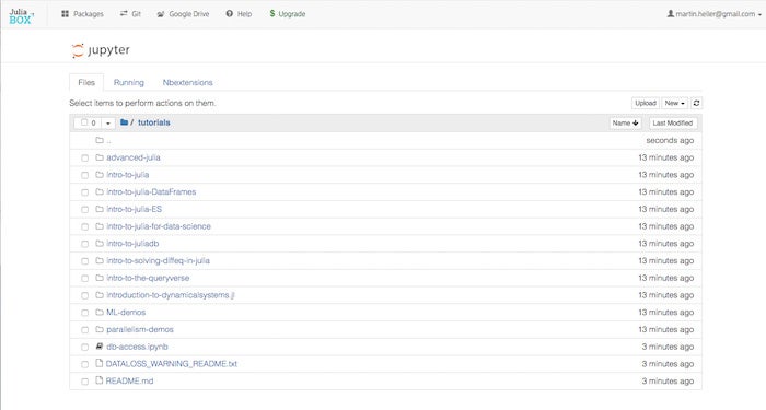
You can run Julia in Jupyter notebooks online using JuliaBox (shown below), another product of Julia Computing, without doing any installation on your local machine. JuliaBox currently includes more than 300 packages, runs Julia 0.6.2, and contains dozens of tutorial Jupyter notebooks. The top-level list of tutorial folders is shown below. The free level of JuliaBox access gives you 90-minute sessions with three CPU cores; the $14 per month personal subscription gives you four-hour sessions with five cores; and the $70 per month pro subscription gives you eight-hour sessions with 32 cores. GPU access is not yet available as of June 2018.
 IDG
IDG
JuliaBox runs Julia in Jupyter notebooks online.
Julia packages
Julia “walks like Python, but runs like C.” As my colleague Serdar Yegulalp wrote in December 2017, Julia is starting to challenge Python for data science programming, and both languages have advantages. As an indication of the rapidly maturing support for data science in Julia, consider that there are already two books entitled Julia for Data Science, one by Zacharias Voulgaris, and the other by Anshul Joshi, although I can’t speak to the quality of either one.
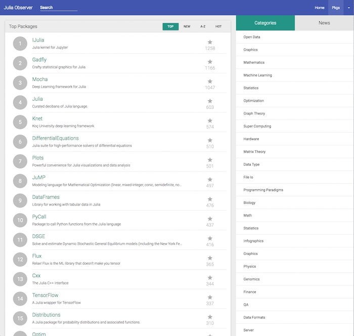
If you look at the overall highest-rated Julia packages from Julia Observer, shown below, you’ll see a Julia kernel for Jupyter notebooks, the Gadfly graphics package (similar to ggplot2 in R), a generic plotting interface, several deep learning and machine learning packages, differential equation solvers, DataFrames, New York Fed dynamic stochastic general equilibrium (DSGE) models, an optimization modeling language, and interfaces to Python and C++. If you go a little farther down this general list, you will also find QuantEcon, PyPlot, ScikitLearn, a bioinformatics package, and an implementation of lazy lists for functional programming.
 IDG
IDG
Julia’s top packages.
If the Julia packages don’t suffice for your needs, and the Python interface doesn’t get you where you want to go, you can also install a package that gives you generic interfaces to R (RCall) and Matlab.
Julia for financial analysts and quants
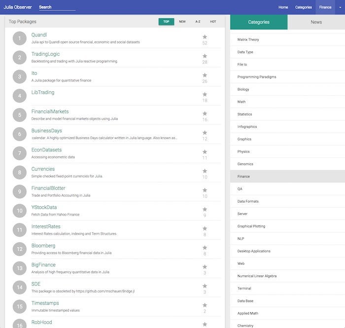
Quants and financial analysts will find many free packages to speed their work, as shown in the screenshot below. In addition, Julia Computing offers the JuliaFin suite, consisting of Miletus (a DSL for financial contracts), JuliaDB (a high performance in-memory and distributed database), JuliaInXL (call Julia from Excel sheets), and Bloomberg connectivity (access to real-time and historical market data).
 IDG
IDG
Julia’s top finance packages.
Julia for researchers
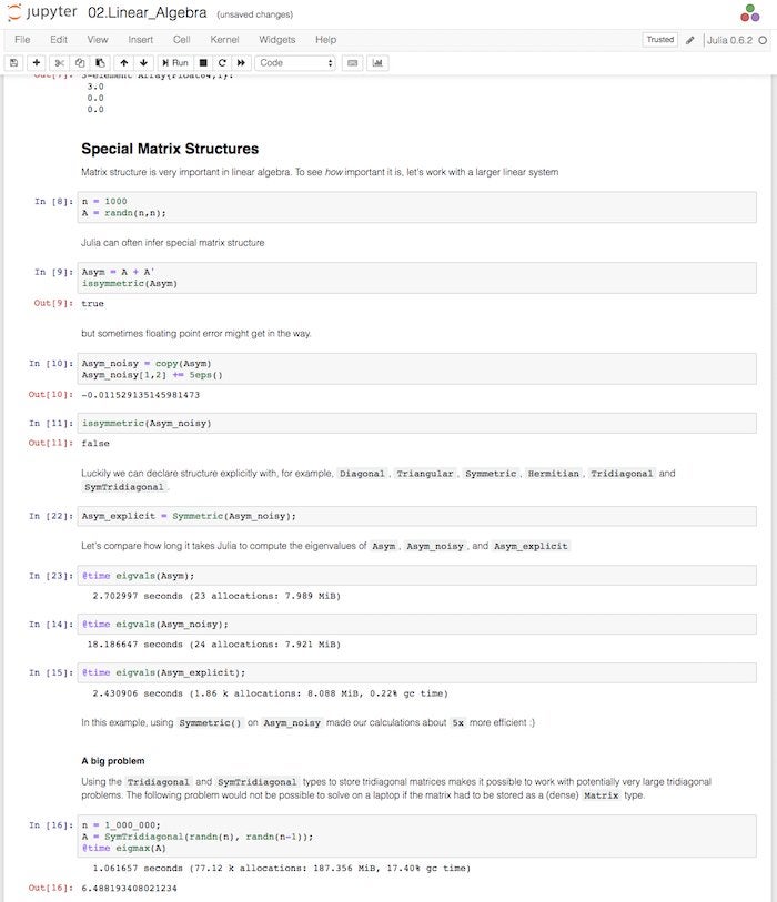
Researchers will find many packages of interest, as you can see from the category names in the right-hand column above. In addition, many of the base features of the Julia language are oriented towards science, engineering, and analysis. For example, as you can see in the screenshot below, matrices and linear algebra are built into the language at a sophisticated level.
 IDG
IDG
Julia offers sophisticated support for multi-dimensional arrays and linear algebra operations.
Learn Julia
As you’ve seen, you can use Julia and many packages for free, and buy enterprise support and advanced features if you need them. There are a few gotchas to consider as you’re starting to evaluate Julia.
First, you need to know that ordinary global variables make Julia slow. That’s because variables at global scope don’t have a fixed type unless you’ve declared one, which in turn means that functions and expressions using the global variable have to handle any type. It’s much more efficient to declare variables inside the scope of functions, so that their type can be determined and the simplest possible code to use them can be generated.
Second, you need to know that variables declared at top level in the Julia command line are global. If you can’t avoid doing that, you can make performance a little better (or less awful) by declaring them const. That doesn’t mean that the value of the variable can’t change—it can. It means that the type of the variable can’t change.
Finally, read the Julia manual and the official list of Julia learning resources. In particular, read the getting started section of the manual and watch Jane Herriman’s introductory tutorial and any other videos in the learning resources that strike you as relevant. If you would prefer to follow along on your own machine rather than on JuliaBox, you may want to clone the JuliaBoxTutorials repo from GitHub and run the Local_installations notebook from Jupyter to install all the packages needed.
Source: InfoWorld Big Data

